Notes: Satisfiability Modulo Theories (SMT)

SAT: Satisfiability for Propositional Logic

Input: For boolean variables $x_1, x_2,\cdots, x_n$, the Clasual Normal Form(CNF) of a clause:

$$(x_1 \vee \neg x_2)\wedge (x_2 \vee x_3) \wedge \neg x_4$$

Terms

• literal: $l = x_i \textrm{ or } \neg x_i$
• clause: $\omega = \bigvee_{l\in \omega} l$
• formula: $\phi = \bigwedge_{\omega\in \phi} \omega$

Assignment:

$$\begin{align}
l^\nu &= \begin{cases}\nu(x_i) & \textrm{if } l = x_i\\ 1 - \nu(x_i) & \textrm{if } l = \neg x_i\end{cases} \\
\omega^\nu &= \max\{l^\nu\ |\ l\in\omega\} \\
\phi^\nu &= \min\{\omega^\nu\ |\ \omega \in \phi\}
\end{align}$$

Output: if the clause is satisfiable.

• Satisfiable (SAT): $\exist \nu (\phi^\nu = 1)$
• Unsatisfiable(UNSAT): $\forall \nu (\phi^\nu = 0)$

DPLL algorithm

Alternate between propagations (assign values to atoms whose value is forced) and decisions (choose an arbitrary value for an unassigned atom)

Example

for clause

$$(x_1 \vee x_2)\wedge (x_3 \vee x_4) \wedge \neg x_2$$

1. Propagate: $x_2$ has to be $0$
2. Propagate: $x_1\gets 1$
3. Decide: $x_3\gets 1$

Clause is SAT

Satisfiability Modulo Theories

"Reasoning about theories"

Replace boolean variable with propositions within theories, e.g. linear integer arithmetics(LIA), string theory

$$(a + 1 > 0 \vee a + b > 0) \wedge (a < 0 \vee a + b > 4) \wedge \neg (a + b > 0)$$

DPLL(T)

Incorporate theory solver with SAT solver.

1. Map variables to clauses:

   $$\phi = (x_1\vee x_2)\wedge(x_3 \vee x_4)\wedge\neg x_2, \\
   \textrm{ where}
   \begin{cases}
   x_1 \Lrarr a + 1 > 0\\x_2\Lrarr a + b > 0\\x_3\Lrarr a < 0\\x_4\Lrarr a + b > 4
   \end{cases}$$

2. Invoke SAT solver

   1. Propagate: $x_2 \gets 0$
   2. Propagate: $x_1\gets 1$
   3. Decide: $x_3\gets 1$

3. Invoke theory (LIA) solver on:

   $$\begin{cases}
   a + 1 > 0\\
   \neg(a + b > 0)\\
   a < 0
   \end{cases}$$

   $x_1$ and $x_3$ are LIA-unsatisfiable

4. add $(\neg x_1 \vee \neg x_3)$ to clauses, Backtrack to last decision

   3. Propagate: $x_3\gets 0$
   4. Propagate: $x_4\gets 1$

5. Invoke LIA solver on:

   $$\begin{cases}
   a + 1 > 0\\
   \neg(a + b > 0)\\
   \neg(a < 0)\\
   a + b > 4
   \end{cases}$$

   $\neg x_2$ and $x_4$ are LIA-unsatisfiable

6. add $(x_2 \vee \neg x_4)$ to clauses, no decision to backtrack, SMT is UNSAT.

Conflict Driven Clause Learning (CDCL)

Unit Propagation: If a clause is unit, then its sole unassigned literal must be assigned value 1 for the clause to be satisfied.

Terms

Each variable is characterized by a number of properties:

• Value: $\nu(x_i) = \{0, u, 1\}$

• Antecedent: $\alpha(x_i) \in \phi \cup \{\rm NIL\}$

  • Only apply for variables whose values are implied by other assignments
  • Means the clause where a variable's value is propagated

• Decision level: $\delta(x_i) \in \{-1, 0, 1, \cdots, |X|\}$

  • The decision level for an unassigned variable $x_i$ is $-1$

  • Means the level of decision tree the variable is at:

    $$\delta(x_i) = \max(\{0\}\cup \{\delta(x_j)\ |\ x_j\in \omega \wedge x_j\neq x_i\})$$

    where $\omega$ is the antecedent of $x_i$.

Example

$$\begin{align*}
\phi &= \omega_1\wedge \omega_2 \wedge \omega_3\\
&= (x_1 \vee \neg x_4)\wedge (x_1\vee x_3)\wedge (\neg x_3 \vee x_2 \vee x_4)
\end{align*}$$

1. Decide: $x_4 \larr 0$, decision level $\delta(x_4) = 1$, Noted as $x_4 = 0 @ 1$.
2. Decide: $x_1 = 0@2$.
   1. Propagate: $x_3 = 1@2$, $\alpha(x_3) = \omega_2$
   2. Propagate: $x_2 = 1@2$, $\alpha(x_2) = \omega_3$

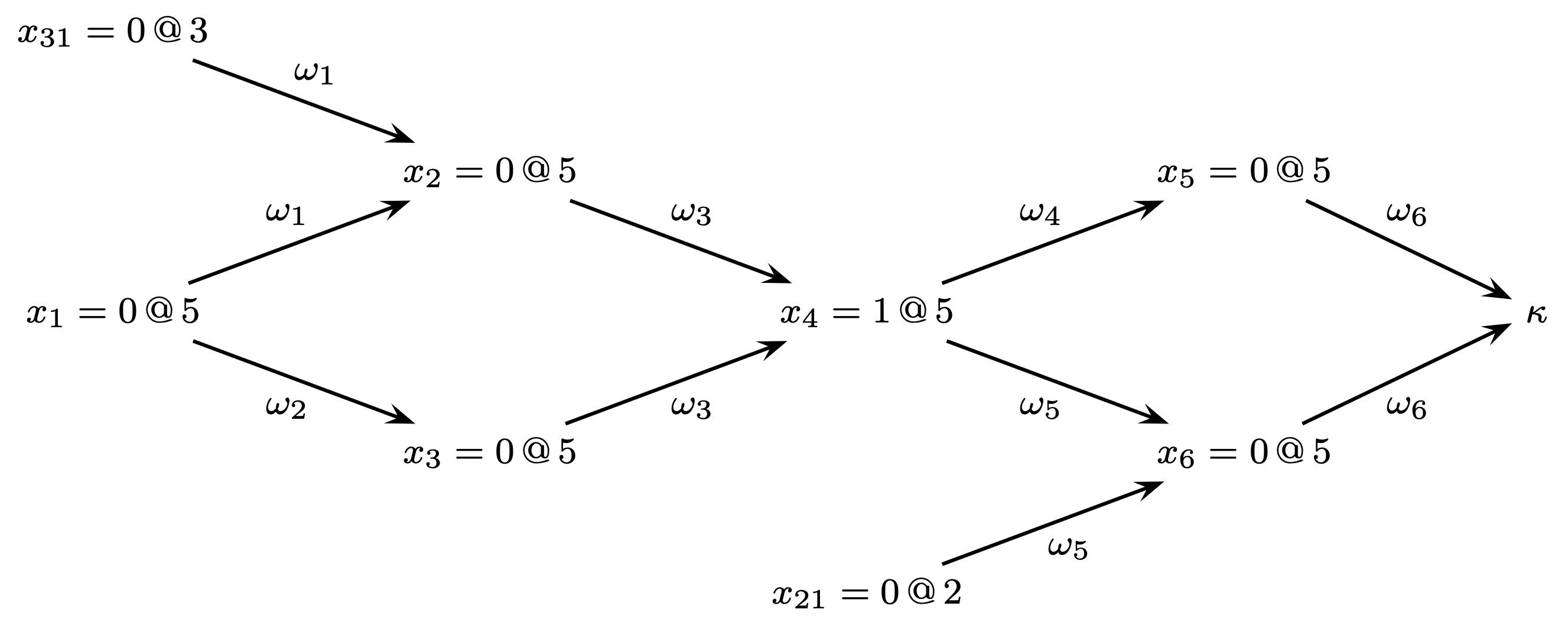
Implication Graph^[1]

$$I = (V_I, E_I)$$

• $V_I$ is all assigned variables, and one special node $\kappa$
  • $\kappa$: If unit propagation yields an unsatisfied clause $\omega_j$, then a special vertex $\kappa$ is used to represent the unsatisfied clause.
• $E_I$: if $\omega = \alpha(x_i)$, then there is a directed edge from each variable in $\omega$, other than $x_i$, to $x_i$.

Algorithm

Algorithm CDCL(φ, ν):
    if (UnitPropagation(φ, ν) = CONFLICT):
        return UNSAT
    dl ← 0                                      # Decision level

    while (¬AllVariablesAssigned(φ, ν)):
        (x, v) = PickBranchingVariable(φ, ν)    # Decide stage
        dl ← dl + 1                             # Increment decision level
                                                # due to new decision
        ν ← ν ∪ {(x, v)}
        if (UnitPropagation(φ, ν) = CONFLICT):  # Deduce stage
            β ← ConflictAnalysis(φ, ν)          # Diagnose stage
            if (β < 0)
                return UNSAT
            else
                Backtrack(φ, ν, β)
                dl ← β                          # Decrement due to backtracking
    return SAT

• UnitPropagation consists of the iterated application of the unit clause rule. If an unsatisfied clause is identified, then a conflict indication is returned.
• PickBranchingVariable consists of selecting a variable to assign and the respective value.
• ConflictAnalysis consists of analyzing the most recent conflict and learning a new clause from the conflict.
• Backtrack backtracks to the decision level computed by ConflictAnalysis.

Learning clauses from conflicts

Notations

• $d$: decision level
• $x_i$: decision variable
• $\nu(x_i) = v$: decision assignment
• $\omega_j$: unsatisfied clause, $\alpha(\kappa) = \omega_j$
• $\odot$: resolution operator:
  • for two clauses $\omega_j$ and $\omega_k$, for which there is a unique variable $x$ such that one clause has a literal $x$ and the other has literal $\neg x$, $\omega_j\odot\omega_k$ contains all the literals of $\omega_j$ and $\omega_k$ with the exception of $x$ and $\neg x$.
• $\xi(\omega, l, d) = l \in \omega \wedge \delta(l) = d \wedge \alpha(l) \neq \textrm {NIL}$: if a clause $\omega$ has an implied literal $l$ assigned at the current decision level $d$
• $\omega^{d, i}_{L}$: the intermediate clause obtained after $i$ resolution operations

$$\omega_L^{d, i} = \begin{cases}
\alpha(\kappa) & \textrm{if } i = 0\\
\omega_L^{d, i - 1} \odot \alpha(l) & \textrm{if } i \neq 0 \wedge \xi (\omega_L^{d, i - 1}, l, d) = 1\\
\omega_L^{d, i - 1} & \textrm{if } i \neq 0 \wedge \forall_l \xi (\omega_L^{d, i - 1}, l, d) = 0\\
\end{cases}$$

$$\begin{align*}
\phi_1 &= \omega_1 \wedge \omega_2 \wedge \omega_3 \wedge \omega_4  \wedge \omega_5 \wedge \omega_6\\
&= (x_1 \vee \neg x_3) \wedge (x_1 \vee  \neg x_3) \wedge (x_2 \vee x_3 \vee x_4) \wedge (\neg x_4 \vee \neg x_5) \wedge (x_{21} \vee \neg x_4 \vee \neg x_6) \wedge (x_5 \vee x_6)
\end{align*}$$

Resolution Steps

1. $\omega_L^{5, 0} = \alpha(\kappa) = \omega_6 = \{x_5, x_6\}$

2. $\omega_L^{5, 1} = \omega_L^{5, 0} \odot \alpha(x_5) = \omega_L^{5, 0}\odot \omega_4 = \{\neg x_4, x_6\}$

3. $\omega_L^{5, 2} = \omega_L^{5, 1} \odot \alpha(x_6) = \omega_L^{5, 1}\odot \omega_5 = \{\neg x_4, x_{21}\}$

4. $\omega_L^{5, 3} = \omega_L^{5, 2} \odot \alpha(x_4) = \omega_L^{5, 2}\odot \omega_3 = \{x_2, x_3, x_{21}\}$

5. repeat until a fixed point occurs: $\omega_L^{5, 6} = \{x_1, x_{31}, x_{21}\}$

6. the learned clause is $\omega_L^5 = (x_1\vee x_{31} \vee x_{21})$

Unit Implication Points ^[1]

A vertex $u$ dominates another vertex $x$ in a directed graph if every path from $x$ to another vertex $\kappa$ contains $u$^[2]. In the implication graph, a UIP $u$ dominates the decision vertex $x$ with respect to the conflict vertex $\kappa$.

• $\sigma(\omega, d) = |\{l \in \omega | \delta(l) = d\}|$: the number of literals in $\omega$ assigned at decision level $d$

$$\omega_L^{d, i} = \begin{cases}
\alpha(\kappa) & \textrm{if } i = 0\\
\omega_L^{d, i - 1} \odot \alpha(l) & \textrm{if } i \neq 0 \wedge \xi (\omega_L^{d, i - 1}, l, d) = 1\\
\omega_L^{d, i - 1} & \textrm{if } i \neq 0 \wedge \sigma (\omega_L^{d, i - 1}, d) = 1\\
\end{cases}$$

Other Clause Learning Algorithms

GRASP^[1]

Apart from conflict analysis, these solvers include lazy data structures, search restarts, conflict-driven branching heuristics and clause deletion strategies.

Nelson-Oppen Theory Combination

SMT with multiple theories

$$f(f(x) - f(y)) = a\\
f(0) > a + 2\\
x = y$$

belongs to Linear Real Arithmetics(LRA) and Uninterpreted Functions(UF)

1. purify literals, each literal should belong to a single theory

   1. $f(f(x) - f(y)) = a$
      • $f(e_1) = a, e_1 = f(x) - f(y)$
      • $f(e_1) = a, e_1 = e_2 - e_3, e_2 = f(x), e_3 = f(y)$
   2. $f(0) > a + 2$
      • $f(e_4) = e_5, e_4 = 0, e_5 > a + 2$
   3. $x = y$

   UF	LRA
   $f(e_1) = a$	$e_1 = e_2 - e_3$
   $f(x) = e_2$	$e_4 = 0$
   $f(y) = e_3$	$e_5 > a + 2$
   $f(e_4) = e_5$
   $x = y$

2. Exchange entailed interface equalities, equalities over shared constants $e_1, e_2, e_3, e_4, e_5, a$

   $x = y, f(x) = f(y)\Rarr e_2 = e_3$

   $e_2 = e_3, e_1 = e_2 - e_3, e_4 = 0 \Rarr e_1 = e_4$

   $e_1 = e_4, f(e_1) = f(e_4)\Rarr a = e_5$

   UF	LRA
   $f(e_1) = a$	$e_1 = e_2 - e_3$
   $f(x) = e_2$	$e_4 = 0$
   $f(y) = e_3$	$e_5 > a + 2$
   $f(e_4) = e_5$	$e_2 = e_3$
   $x = y$	$a = e_5$
   $e_1 = e_4$

Nelson-Oppen (non-deterministic, non-incremental)

Notations:

• $T_i$: first-order theory of signature $\Sigma_i$, set of function and predicate symbols in $T_i$ other than $=$
• $T = T_1\cup T_2$
• $C$: a finite set fo free constants, i.e. not in $\Sigma_1 \cup \Sigma_2$
• $L_i$ finite set of ground (i.e. variable-free) $(\Sigma_i \cup C)$-literals

Input: $L_1 \cup L_2$

Output: SAT or UNSAT

1. Guess an arrangement $A$, i.e., a set of equalities and disequalities over $C$ such that:

$$\forall c, d\in C (c = d\in A \vee c\neq d \in A)$$

2. If $L_i\cup A$ is $T_i$-UNSAT for $i \in \{1, 2\}$, return UNSAT
3. return SAT

The algorithm is terminating, sound and complete under certain conditions($\Sigma_1\cap \Sigma_2 = \varnothing\wedge T_1, T_2$ are stably infinite)

• when the method returns sat for some arrangement, the input is SAT.

References

[1] J. P. Marques-Silva and K. A. Sakallah. GRASP: A new search algorithm for satisfiability. In International Conference on Computer-Aided Design, pages 220–227, November 1996.

[2] R. E. Tarjan. Finding dominators in directed graphs. SIAM Journal on Computing, 1974.

× ← →